Getting Started
Assuming that your WASS installation was successful this tutorial will let you run the pipeline to reconstruct some sample real-world sample data. This should help you acquire familiarity with some of the concepts that will be expanded in the following parts of the documentation.
WASS architecture
WASS is composed by a set of program executables that perform, in sequence, specific steps of the reconstruction process (that's why is called a pipeline).
An external process, called WASSjs, controls the execution of such pipeline to provide a simple graphical web-based user interface to the user and exploit the best possible parallelism offered by modern multi-core machines.
At the moment, WASS is composed by the following programs (you can see them under <WASS_ROOT>/dist/bin/):
| Name | Task |
|---|---|
wass_prepare |
Takes a couple of stereo images as input and place them into a proper "working directory". Images are also undistorted according to the provided intrinsic calibration data |
wass_match |
Matches corresponding features of a stereo image pair. After the matching, the Essential matrix is recovered and the extrinsic parameters between the two cameras are factorized (up to translation scale). Matched features are filtered according to epipolar consistency. |
wass_autocalibrate |
Matches between multiple stereo frames are all collected and Sparse Bundle Adjustment (SBA) is used to simultaneously optimize the extrinsic camera parameters and the 3D points triangulated from all the matches. Final extrinsics are saved to all the workspaces. |
wass_stereo |
Performs dense stereo 3D reconstruction on a given stereo frame. After the reconstruction, multiple filters are applied to the point cloud to remove outliers. Finally, a plane is robustly fitted to the point cloud. |
wass_match and wass_autocalibrate are only used if auto-calibration is needed (ie. the extrinsic parameters are unknown). With the exception of wass_autocalibrate that operates on all the working directories simultaneously, each program loads its data from a specific working directory and saves its results into that.
The "working directory" is a basic unit of work that holds two corresponding stereo frames together with the computed reconstruction data (point cloud, plane parameters, etc). All the working directories of a stereo sequence follows the following name convention:
000000_wd/ for the first frame, 000001_wd/ for the second, and so on. No assumption are made on the temporal difference between two frames that are all considered independent and hence processed in parallel.
Note for multi-core/cpu platforms
Each wass component (ie. wass_stereo, wass_match, etc.) runs as a
single-threaded process performing a specific task on a working directory. To
exploit the intrinsic parallelism of the stereo reconstruction task, the WASSjs
controller manages multiple parallel instances of each component.
As a consequence, WASS can scale well in distributed memory machines (like virtualized environments) with the only requirement to have a consistent shared view of a common filesystem.
How to run it
If you skipped the testing step, please download the data from
http://www.dsi.unive.it/wass/WASS_TEST.zip
and unzip the downloaded package into the <WASS_ROOT>/test directory. That package also contains the sample stereo sequence we are going to process.
In <WASS_ROOT>/test/W07/ you can see how an hypotetical image sequence should be prepared for the reconstruction. The config/ subdirectory contains the calibration data (at least the intrinsics) and some configuration files. The input/ subdirectory contains the image data, divided between the two cameras, whose name convention follows the rule:
<sequence_number (6 digits)>_<timestamp (13 digits)>_<camera number (2 digits)>.tifIn our case, the input/ subdirectory looks as follows:
├── cam0
│   ├── 000000_0000000000000_01.tif
│   ├── 000001_0000000083342_01.tif
│   ├── 000002_0000000166652_01.tif
│   ├── 000003_0000000249994_01.tif
│   ├── 000004_0000000333336_01.tif
│   └── 000005_0000000416678_01.tif
│   └──  ...
└── cam1
    ├── 000000_0000000000000_02.tif
    ├── 000001_0000000083341_02.tif
    ├── 000002_0000000166650_02.tif
    ├── 000003_0000000249991_02.tif
    ├── 000004_0000000333333_02.tif
    └── 000005_0000000416674_02.tif
    └──  ...
After the installation, WASS is pre-configured to reconstruct the sequence
inside <WASS_ROOT>/test/W07/. To launch WASSjs (the pipeline monitor),
execute the following commands, depending on your platform.
On Linux / Mac OSX
Open two terminals. On the first one type:
$ cd <WASS_ROOT>/WASSjs/ext/
$ ./launch_redis.sh
on the second one enter the commands:
$ cd <WASS_ROOT>/WASSjs
$ node Wass.js
WASSjs is now running. Keep both the terminals open during its whole execution.
On Windows
Open <WASS_ROOT>/WASSjs and double click on launch_wassjs.bat. Two
command prompts will appear to show debug informations during WASS execution.
Step 1 - Access WASSjs
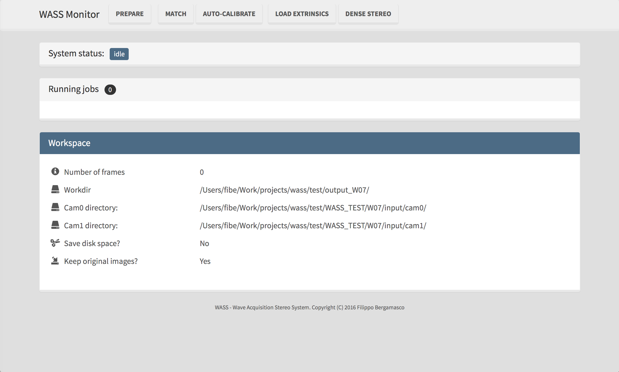
Open your browser at the address http://localhost:8080 to access the wass monitor:
Step 2 - Prepare the working directories
From the top menu, click on PREPARE to start the workspaces preparation process. After a while, the system status will return to idle and a new prepared status should be marked in green.

If you look inside the <WASS_ROOT>/test/WASS_TEST/output_W07/ you should see that a new directory has been created for each input stereo pair.
Step 3 - Auto-calibrate the stereo cameras
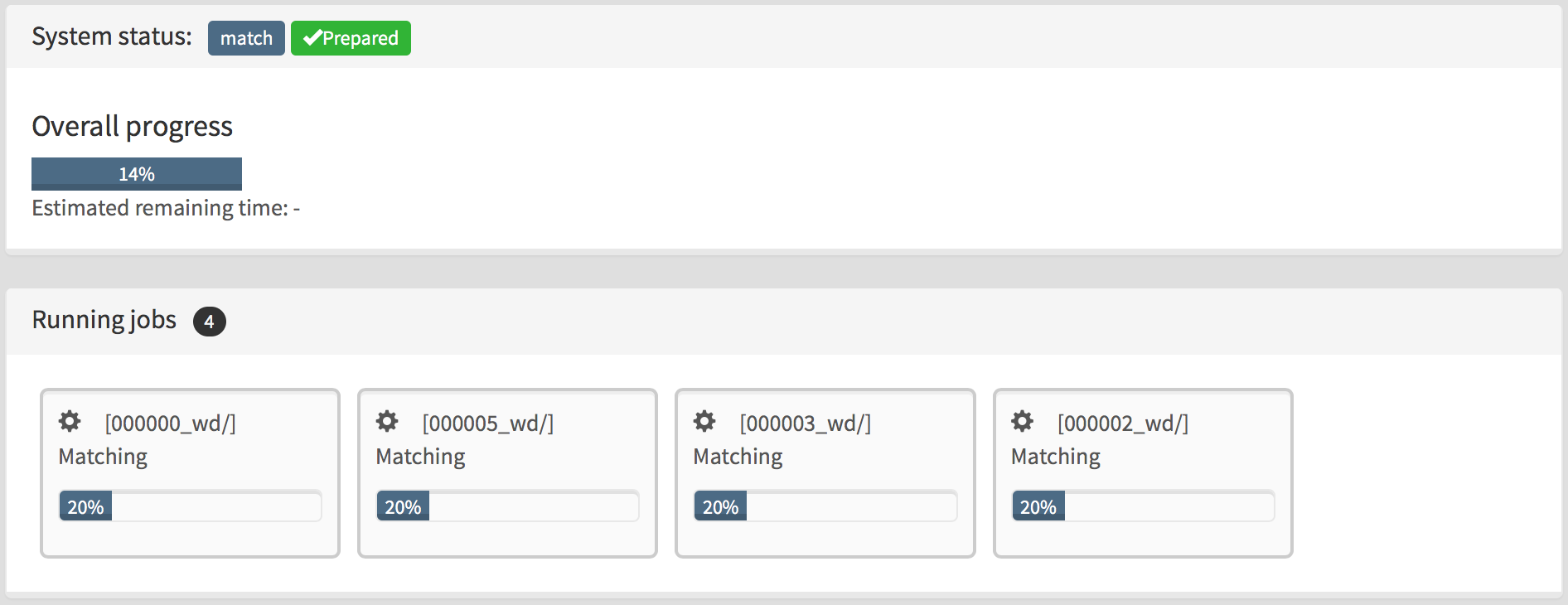
To proceed with the extrinsic calibration of the stereo cameras click on MATCH command on the top menu. WASSjs will start the initial matching step between all the stereo pairs. During the processing, the "overall progress" is displayed in the central part of the page, together with a list of the currently running processes.
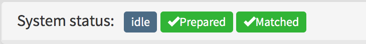
When the match is completed, the system will return to idle status and a new matched status will be marked in green.
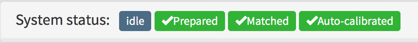
At this point, click on AUTO-CALIBRATE on the top menu to perform the final auto-calibration step. As usual, the system status will be updated show that the cameras are now calibrated.
Step 4 - Run the 3D reconstruction
To reconstruct the stereo sequence, click on DENSE STEREO on the top menu. If the whole process is successful, the final system status will be the following:

Examining the results
At this point, in the output directory <WASS_ROOT>/test/WASS_TEST/output_W07/ you should see all the processed data frames as different zip files.
output_W07
├── 000000_wd.zip
├── 000001_wd.zip
├── 000002_wd.zip
├── 000003_wd.zip
├── 000004_wd.zip
├── 000005_wd.zip
├── autocalibrate.txt
├── worksession.json
└── workspaces.txt
Unzipping one of the working directory, for example 000000_wd/, we should see the following:
000000_wd
├── 00000000_features.png
├── 00000000_s.png
├── 00000001_features.png
├── 00000001_s.png
├── Cam0_poseR.txt
├── Cam0_poseT.txt
├── Cam1_poseR.txt
├── Cam1_poseT.txt
├── K0_small.txt
├── K1_small.txt
├── P0cam.txt
├── P1cam.txt
├── densestereolog.txt
├── disparity_coverage.jpg
├── disparity_final_scaled.png
├── disparity_stereo_ouput.png
├── ext_R.xml
├── ext_T.xml
├── graph_components.jpg
├── intrinsics_00000000.xml
├── intrinsics_00000001.xml
├── matcher_stats.csv
├── matches.png
├── matches.txt
├── matches_epifilter.png
├── matchlog.txt
├── mesh.ply
├── mesh_cam.xyzC
├── plane.txt
├── plane_refinement_inliers.xyz
├── scale.txt
├── stereo.jpg
├── stereo_input.jpg
├── undistorted
│   ├── 00000000.png
│   ├── 00000000_P0.png
│   ├── 00000001.png
│   └── 00000001_P1.png
└── wass_stereo_log.txt
Here is a brief description of the relevant files produced by the wass pipeline for each stereo frame:
| File | Content |
|---|---|
| mesh_cam.xyzC | The reconstructed point cloud as a wass compressed binary mesh format. Use the provided <WASS_ROOT>/matlab/load_camera_mesh.m matlab script to load it into a Matlab matrix |
| mesh.ply | The reconstructed point cloud in PLY format to be easily viewed with MeshLab NOTE: this file is for debug only. The point cloud data to be used for further processing is mesh_cam.xyzC or mesh_cam.xyz |
| Cam0_poseR.txt Cam0_poseT.txt |
Pose of the camera 0, ie. the rotation matrix and translation vector that transform the reconstructed point cloud from the world reference frame to the Cam0 reference frame. |
| Cam1_poseR.txt Cam1_poseT.txt |
Pose of the camera 1, ie. the rotation matrix and translation vector that transform the reconstructed point cloud from the world reference frame to the Cam1 reference frame. |
| intrinsics_00000000.xml | Cam0 intrinsic parameters |
| intrinsics_00000001.xml | Cam1 intrinsic parameters |
| ext_R.xml ext_T.xml |
Extrinsic parameters of the stereo rig. |
| wass_stereo_log.txt | Log produced by wass_stereo. Contains informations on the number of reconstructed points, the filtering process, etc. |
| stereo.jpg | 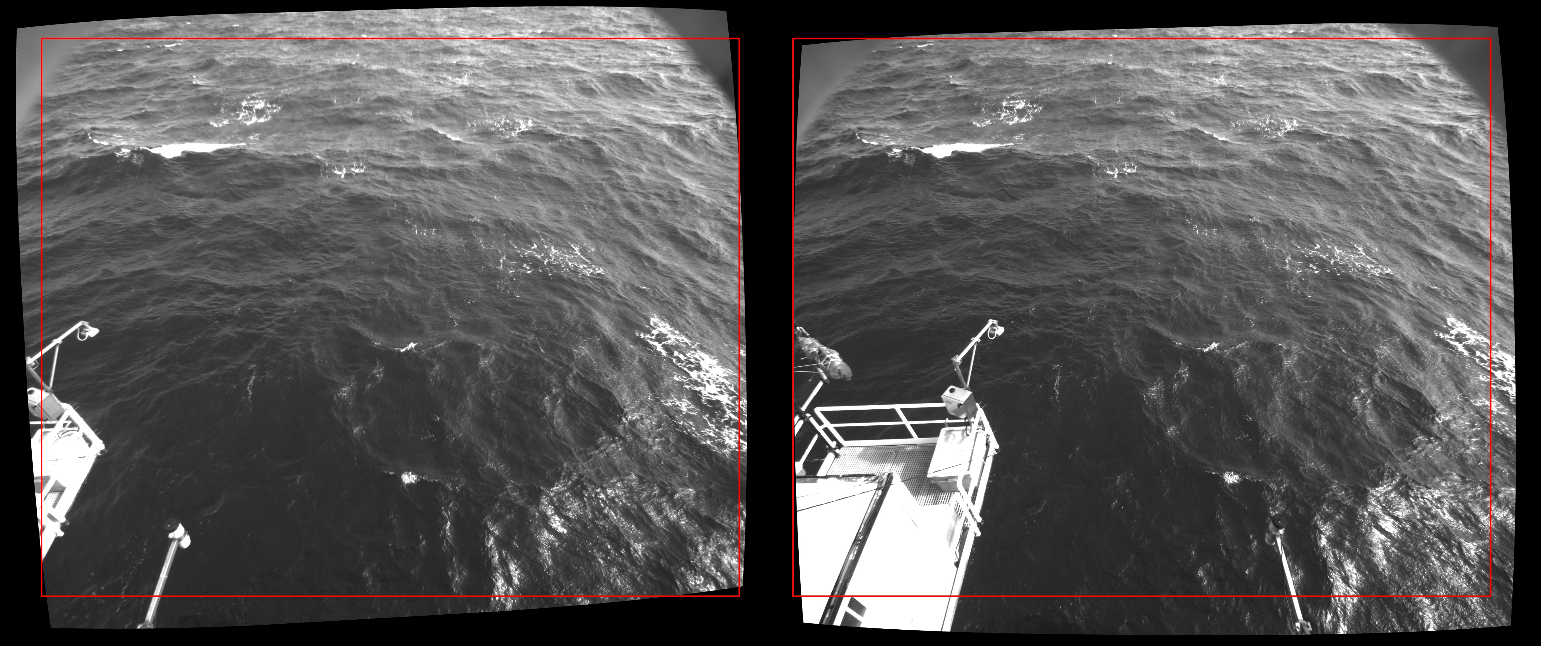 Rectified stereo frames with the computed region of interest. This image is useful to check if all the matching visual features lie on the same image row Rectified stereo frames with the computed region of interest. This image is useful to check if all the matching visual features lie on the same image row |
| disparity_stereo_output.png | 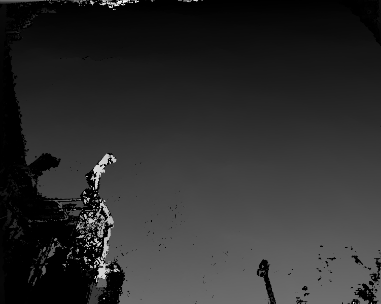 The computed unfiltered disparity matrix The computed unfiltered disparity matrix |
| disparity_final_scaled.png | 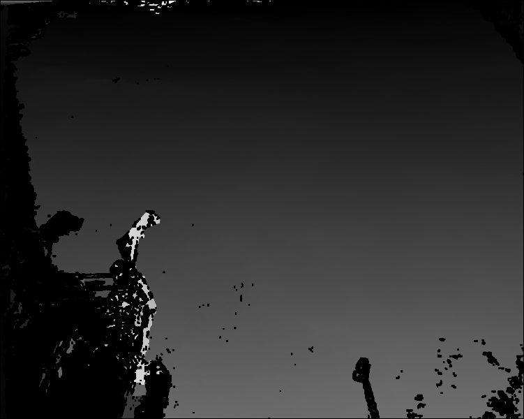 The computed disparity matrix after disparity filtering The computed disparity matrix after disparity filtering |
| disparity_coverage.jpg | 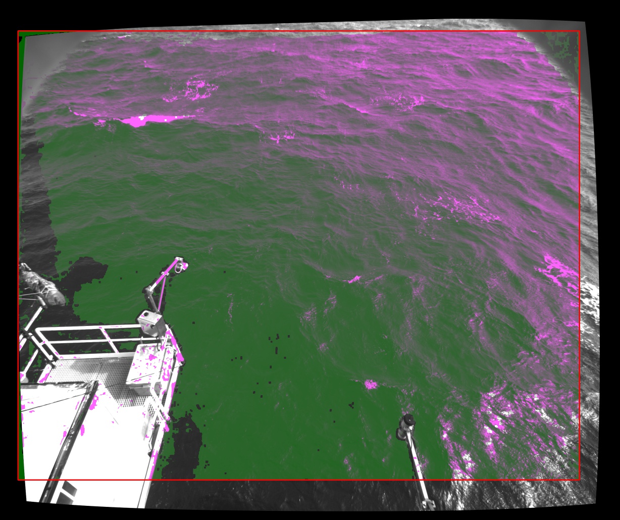 Disparity matrix superimposed to one of the input images Disparity matrix superimposed to one of the input images |
| graph_components.jpg | 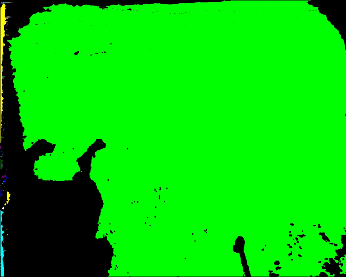 Connected components extracted from the point cloud graph. All but the green one are considered outliers Connected components extracted from the point cloud graph. All but the green one are considered outliers |
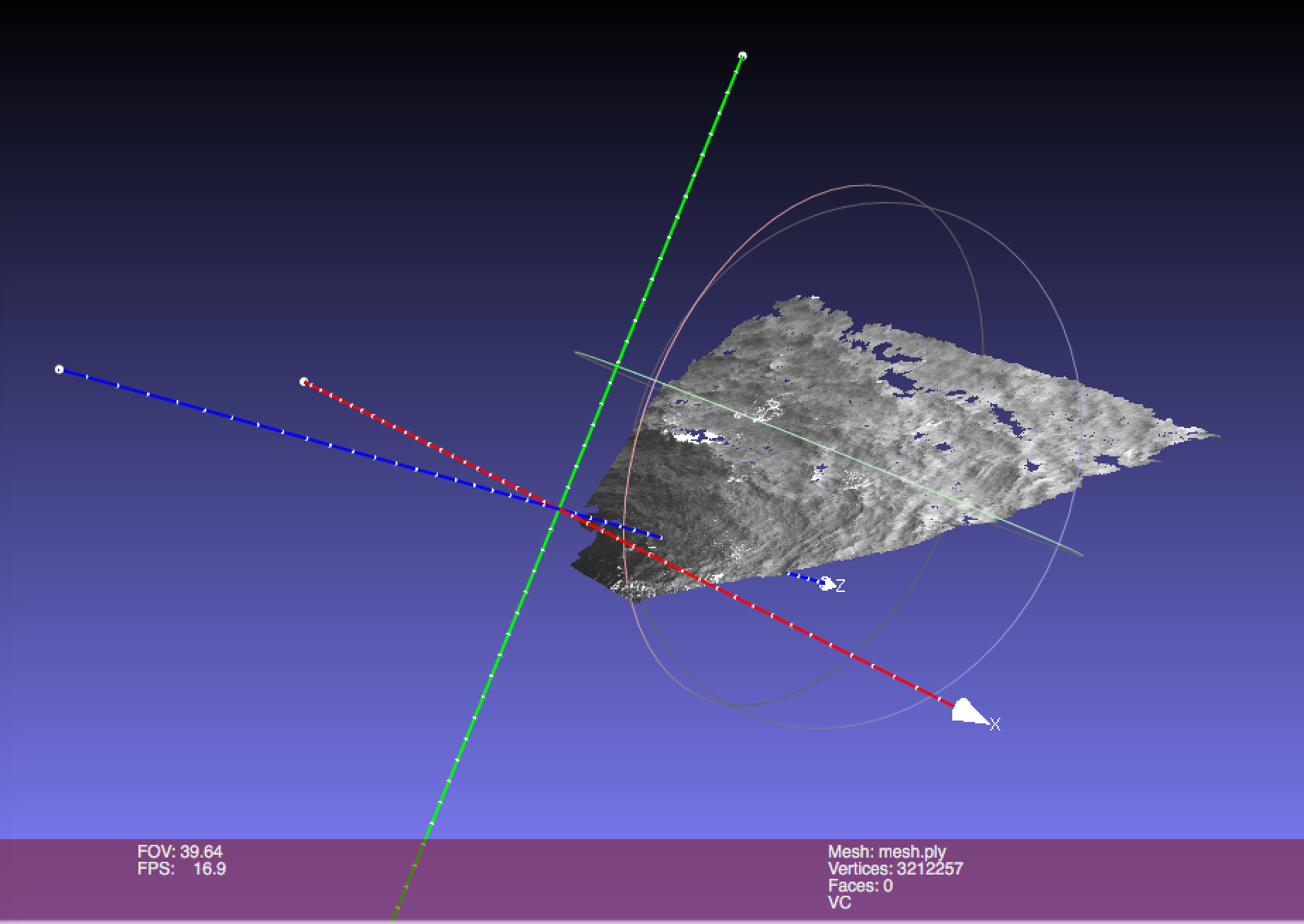
To quickly inspect the reconstructed point cloud for the first stereo frame, download the MeshLab viewer and open 000000_wd/mesh.ply:
Post-Process the 3D point data
An example of how to load and post-process the produced point cloud data is shown in <WASS_ROOT>/test/plot_sequence.m